Grounded Sensitivity
While sensitivity analysis will allow you to explore any sets of assumptions, it is often useful to ground that exploration in history. Stella supports a work flow that starts with Calibration then uses sensitivity to explore confidence bounds on parameters, historical behavior and future projections. The steps are very straightforward, though like most modeling work some amount of iteration will likely be necessary.
- Calibrate the model to historical data following the description in Calibration. Be sure to select the option to automatically adjust the weights. After getting results that you find satisfactory, perform one additional calibration and check the weights (reported in the optimization log) to be sure they are not changing very much. the weights are reported in Optimizer Messages.
- Create a sensitivity run using the same parameters that you used for the calibration. If you set the minimum and maximum for those values in theScales and Ranges Tab the sensitivity run will use those. Select a uniform distribution and use Sobol sequencing selection and at least 100 runs (since iteration is likely you may want to start with 100 runs and then make more once everything has settled down).
- In the Sensitivity Specs Panel set up the criteria for Grounded Sensitivity. Use a relative payoff threshold of 2 (for 95% confidence intervals) and adjust sensitivity parameters with a multiple of 1. More details on the steps involved are included in the example below. When selecting a threshold 2x the payoff is chi-Square with 1 degree of freedom, so you can select the threshold value by picking a confidence level from the percentile tables for that distribution and dividing by 2 (95% is 3.84 rounded to 4 divided by 2 is 2).
- Run the sensitivity. You should target between 10% and 50% of the runs to be successful. To get more successful runs tight the bounds (for example instead of 1 for a multiplier use 0.75), to get fewer make the bounds wider.
- After you get about the right number of runs, set the bounds more explicitly using the content and recommendation in the Message Log. Except when a parameter is physically bounded below or above, you should be selecting a range so that the minimum or maximum would never succeed no matter what values the other parameters take on. The recommended values are 1.5 times the distance from the realized minimum and maximum relative to the base value.
- The resulting set of successful runs will allow you to see distributions for the optimization parameters, historical behavior of all model variables, and project behavior consistent with that historical behavior.
Note A good way to get the parameters for both optimization and sensitivity into their respective specifications is to use tags set in the Documentation Tab as shown in the example below.
Successful Simulations
The set of simulations that meet the criteria provide you with a multivariate distribution of the parameters that are consistent with historical data. It is easy to look at the distribution of any one of those parameters using a Bar Graph configured to show a histogram across runs.
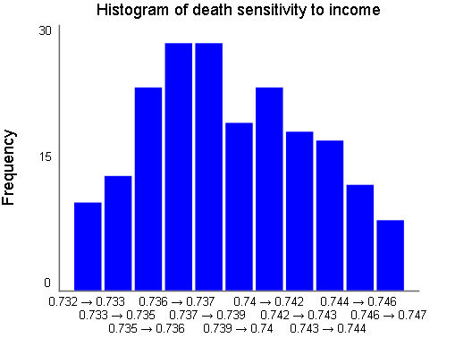
More importantly, the joint distribution of all parameters is implicitly used in the successful simulation. You can pull out the parameters to determine the characteristics of that n-dimensional distribution in other tools, but the sensitivity results displayed are automatically a consequence of that join distribution.
Example
In this example we will work through both the calibration and grounded sensitivity process starting from a model and some data. It is a small model that hes been set up with make the steps that follow very straightforward. You can also view this example as a video here.
Download the model GroundedSensitivity.stmx and the csv file GroundedSensitivity.csv that goes with it.
- Open the model.
- Import the csv file as a run by opening the Data Manager and clicking on
 in the bottom left and selecting the GroundedSensitivity.csv file.
- Run the model and look at the comparative graph. You can select any of the output variables from the dropdown above it. The model and data are quite different.
- Set up a payoff by opening Payoff Specs, select Calibration as the type and select GroundedSensitivity as the comparison run. Then click on the
 below Payoff Elements and in the Find window selecting tagged with Output, clicking on Select All and then OK. there should be 4 items in the list.
- Setup an optimization by opening Optimization Specs, selecting Payoff as the payoff then clicking on the below the Optimization Parameters list and selecting everything tagged with Parameter. Because the parameters already have bounds from the Scales and Ranges Tab you don't need to do anything else.
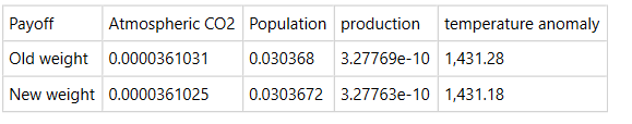
- Click on the run button, see the change in the output. Look at the log to see the weights chosen.
- Click on the O-Run button in the bottom left a few more times. Notice that the results are changing only a little bit, and the weights get fairly stable. The weights for temperature anomaly converge the most slowly.
- In the model change the variable calibration switch to have value 0. This is used in setting the models stop time.
- Open the Sensitivity Specs Panel and add the same variables use for optimization - those tagged as Parameter. Set the number of runs to be 100
- Click on the Setup Criteria button for Grounded Sensitivity. Use the default of 2 and relative, then check the Adjust sensi parameters button and click OK.
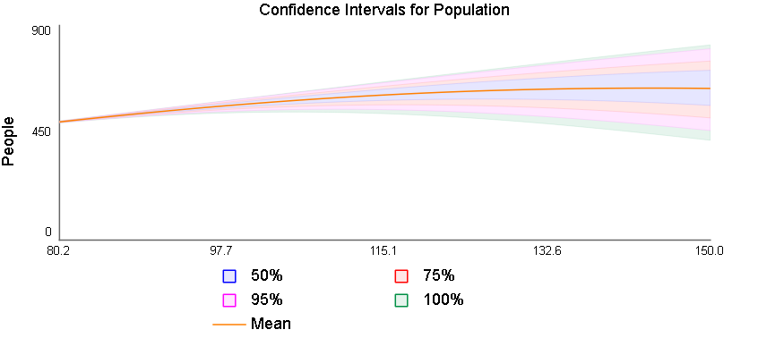
- Click on run in the panel. Then look at the graph - for example for population:
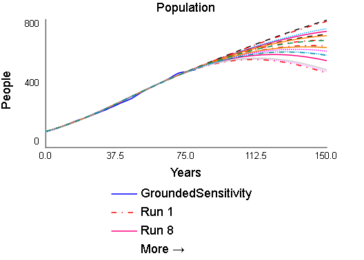
The historic or grounding period shows little variation. The projection period shows more
- Look at the information in the message log to make adjustments to parameter ranges.
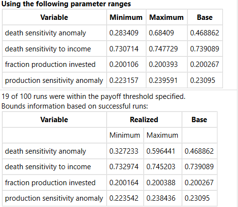
Make sure the ranges selected are broader than those that realized accepted outcomes. A rule of thumb is half again the distance from the base values.
- Once
you have a satisfactory set of parameter ranges, increase the number of simulations so that you can get sensitivity results that are displayed using the Bar Graph or Confidence Graph.
The historic or grounding period shows little variation. The projection period shows more.